Posted June 28, 2021

Geotechnical instrumentation suppliers often use off the shelf MEMS sensors and typically apply some in-house calibration and sample averaging to help increase the precision of the readings in various environmental conditions.

As discussed in Session 01, precision is one of the most important parameters, and is commonly presented in the specifications in units of arcseconds, degrees, or mm/m. Conditions that can impact precision in the field include the following:

• Temperature (both absolute and change in temperature)
• Sample averaging rate (some manufactures allow you to change this to balance precision and power consumption)
• Inclination (specified precision is typically based on vertical orientation. As the tilt from vertical increases, the precision may decrease)
• Mechanical relaxation (slight movements of the mechanical components in the casing due to material creep, loading, and/or temperature change)
• Duration of measurements (precision is typically specified over a duration: 24 hours, 7 days, etc. MEMS have some time dependent uncertainty, sometimes described as drift or long term stability, which may need to be taken into account depending on the duration of the project).

A practical application of precision is looking at a set of in-place inclinometer (IPI) data over a period of time, and trying to determine if the data is showing actual ground movement, or if the output movement is associated with the cumulation of errors in the instrument or system itself. These errors could be sensor (associated with the MEMS and other electronic components) or mechanical (ie. the instrument is moving in the casing, but the casing itself is not moving).

Incremental Displacement Example (detecting movement at a specific instrument location):

The plot below shows field data from a single IPI installed 20 feet below ground (temperature is stable at this depth). The plot shows data collected at 5 minute intervals over the span of approximately 3 months. Sample averaging is done at the board level and the output represents average readings over 800 samples. The stated resolution of the sensor is ±0.004 mm/m which is likely being met in all cases, however this parameter is not very helpful in determining if real movement is occurring. The stated precision value of the sensor is ±0.13 mm/m over a 99% confidence interval, which this particular instrument is meeting (the data generally falls within ±0.1 mm/m). In this case as the data is not showing a trend in either the positive or negative direction, and all data is within the precision specification of the sensor, it is a generally accepted interpretation that no movement is occurring at this IPI location.

Cumulative Displacement Example (detecting movement at the ground surface):

Now that we have a good understanding of the sensor performance in an individual instrument, how can this information be extrapolated to a string of IPI’s and applied to cumulative displacement data to interpret movement at the ground surface?

One way of estimating the cumulative system error is to calculate an error band based on the number of sensors in the string. This can be accomplished by taking the square root of the sum of the squares of all of the errors associated with the system.

As an example: a string of 10 IPI’s spaced continuously at 10 ft in a borehole to a total depth of 100 ft. The sensor specifications are as follows:

• Resolution: ±0.0002°
• Precision: ±0.0050°
• Nonlinearity: ±0.0020°
• Temperature Dependent Uncertainty: ±0.0040°/°C

The first IPI sees a temperature fluctuation of 7°C and the second IPI sees a temperature fluctuation of 3°C. The remaining 8 IPI’s are deep enough to avoid temperature effects from surface temperature changes. The incremental error band associated with IPI 1 can be estimated as follows:

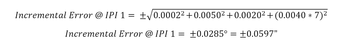
Calculating the incremental error for each IPI and then plotting the cumulative error band alongside some sample IPI data yields the following results:

Without the error bands one may interpret that the surface is moving over 0.05 in, however with the known errors associated with the sensors plotted alongside the IPI data, you can easily see that the output is within the error of the system, and the movement is likely associated with the cumulative error of the system, in particular the temperature dependent uncertainty seen by the top instrument.

Disclaimer: This article is intended for information purposes only in an attempt to explain the various terms used in MEMS based instruments and is not intended to be used as engineering judgement for interpretation of displacement data at any particular site and/or with any particular system.

‹ Session 01 • Session 03 ›